
Reinforcement Learning: The Future of Smart Trading
Building an Adaptive Trading Bot With Reinforcement Learning

Hello, coders and investors! Welcome to another edition of Investor’s Edge! Today, we’ll be deep diving into the art of Reinforcement learning and how it can help traders just like you optimize their investment strategies. Whether you’re looking to discover new stock strategies or get started with real-world coding, we hope that you’ll gain an understanding of how to use the methods involved in reinforcement learning to find opportunities.
Let’s get started!
Terms and Conditions
So, what is Reinforcement learning?
Reinforcement learning (RL) involves an agent learning to make decisions by interacting with an environment, seeking to maximize cumulative rewards over time. Unlike supervised learning, which relies on labeled datasets to guide a model to the correct output, RL learns through exploration and feedback, improving its strategy based on successes and failures. In unsupervised learning, there are no labels or explicit guidance; the goal is to uncover hidden patterns or groupings within data. While supervised learning teaches from examples and unsupervised learning searches for underlying structures, RL focuses on learning optimal behaviors through dynamic experience and trial-and-error exploration.

To learn more about RL, read below:
Today, we’ll be using RL strategies to create a trading bot that learns to optimize its stock positions dynamically, using live market data to decide when to buy, sell, or hold shares of Apple. By leveraging the Deep Q-Network algorithm, our bot will interact with a simulated market environment, continuously improving its decision-making over thousands of timesteps. This approach aims to demonstrate how reinforcement learning can be applied to financial trading for maximizing net worth through strategic actions.
To ensure you are able to carry out and run this code on your own device, be sure to determine and install any coding program on your device.
One of the most popular coding platforms is Visual Studio (VS) Code, which you can learn how to install here:
Let’s begin coding!
Step-by-Step Breakdown
Step 1: Set up Your Python Environment
The first step in the process is to initialize our coding environment so that we can get our code to do what we want it to! Python is complex - naturally, coders end up using certain aspects of the language more than others. Other individuals have combined these aspects into mini-programs called libraries. Anyone can install and use these libraries, and they allow us to be as optimal as possible without recreating the systems.
For this project, we’ll need the following libraries:
gymnasium (for data manipulation)
numpy (to compute with arrays)
pandas (to manipulate data frames)
matplotlib (to plot charts)
stable_baselines3 (to train reinforcement models)
yfinance (to fetch stock data)
If this is your first time using these libraries on VS code, you’ll need to install them. Unlike our actual code, we ARE NOT going to run this in the shell. Instead, we install libraries by running them in the terminal. In the image below, the terminal is highlighted in red.
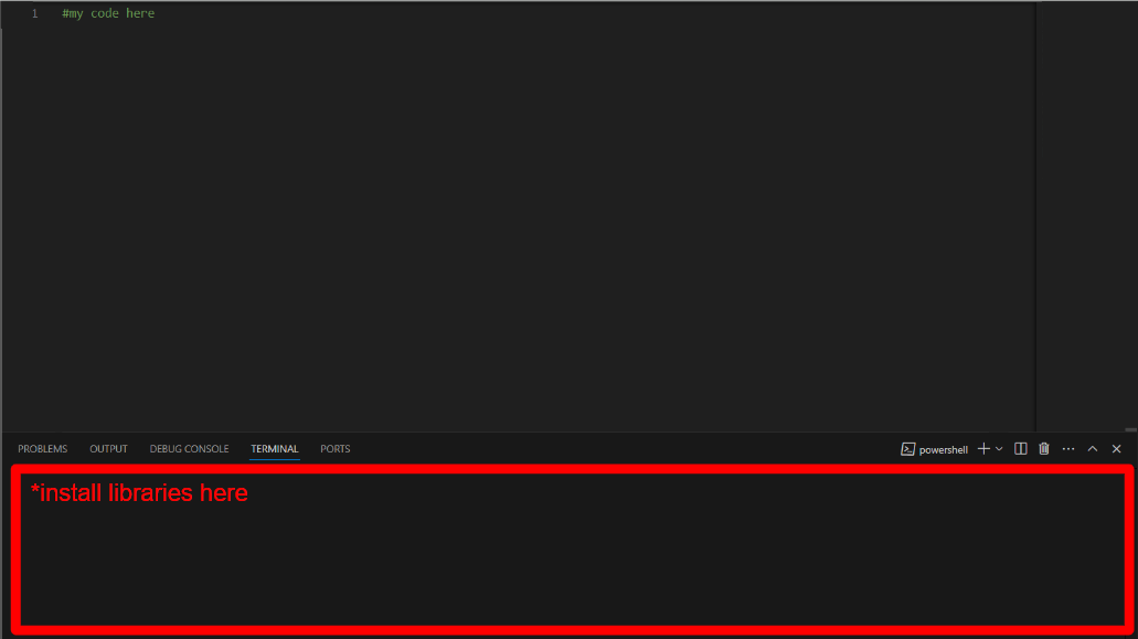
Note: If you’ve already installed these libraries, you can skip this step.
Use the following syntax in your terminal:
import gymnasium as gym
from gymnasium import spaces
import numpy as np
import pandas as pd
import matplotlib.pyplot as plt
from stable_baselines3 import DQN
import yfinance as yf
Step 2: Create the Custom Trading Environment
2.1: Define Environment Class - header size 4
This section initiates the code by creating a custom trading simulation environment using OpenAI’s Gym Library - this is a toolkit used to develop and RL environments. This code can be run in an IDE or directly in an OpenAI platform, like ChatGPT. We beign by creating a custom trading environment, ‘SimpleTradingEnv’ made to work with the Gym library. Inside this class, we proceed by defining a function that initiates the environment where an instance of ‘SimpleTradingEnv’ is created. This is called the constructor of the class. The function accepts the ‘ticker’ parameter, which takes the stock ticker symbol we want to work with, and establishes its initial balance to be $10,000.
Note: Throughout the code, we’ll see many instances of ‘self’. In python, ‘self’ is a reference to the current instance of the class that is in use.
Take a look at the following syntax:
class SimpleTradingEnv(gym.Env):

    def __init__(self, ticker, initial_balance=10000):
We continue by initializing the superclass of ‘SimpleTradingEnv’, which sets up the Gym Environment’s internal structures, with the following code:
super(SimpleTradingEnv, self).__init__()Here’s where we get into some of the more basic code as we define the instance variables. This is rather straightforward; the ‘self.ticker’ stores the corresponding ticker, ‘self.initial_balance’ sets the initial balance, ‘step.current_step’ tracks the steps (amounts of time passed) starting at 0, ‘self.balance’ tracks the current cash balance in the trading account, ‘self.positions’ represents the number of stocks held by the agent, ‘self.net_worth’ is the total net worth of the agent, and ‘self.data’ calls the method ‘_get_live_data()’ - this retrieves dynamic stock data (note that this function has not been defined yet). Here’s the corresponding code:
        self.ticker = ticker

        self.initial_balance = initial_balance

        self.current_step = 0

        self.balance = initial_balance

        self.positions = 0

        self.net_worth = initial_balance

        self.data = self._get_live_data()
Here’s where we define the action space - this is what defines the actions the agent can take while trading. In this case, it’s a discrete space with three possible actions: Buy, Sell, or Hold. After this, we get into the observation space, which is where the coder can explore the possible observations. In our code, it's a continuous box space that defines four inputs: ‘low’, ‘high’, ‘shape’, ‘dtype’. The first two parameters define the minimum and maximum of the observation space, letting the algorithm know that the observation can be any real value. The ‘shape’ parameter suggests that the observation is a single scalar value and ‘dtype’ defines the observation as a 32-bit floating number.
Take a look at the syntax below:
        self.action_space = spaces.Discrete(3)

        self.observation_space = spaces.Box(low=-np.inf, high=np.inf, shape=(1,), dtype=np.float32)
Let’s continue.
2.2: Fetch Stock Data
This next section of the definition of the ‘_get_live_data’ function that we called in the previous substep. This function takes one parameter, ‘self’, which it uses to work with the live, current data dynamically. When this function is called, the algorithm carries out the following:
Prints a confirmation message
Gathers minutely dynamic data for the previous day
Drops the closing price column from the dataset
Normalizes the data
Returns the entire dataset
Let’s dive into this code:
    def _get_live_data(self):

        print(f"Fetching live data for {self.ticker}...")

        stock_data = yf.download(self.ticker, period="1d", interval="1m")

        stock_data = stock_data[['Close']].reset_index(drop=True)

        stock_data = (stock_data - stock_data.mean()) / stock_data.std()

        return stock_data
Looking at the third line in the function, we select only the ‘Close’ column from the ‘stock_data’ DataFrame, discarding all other columns. Then, it resets the index of the DataFrame to create a new, sequential index, ignoring the original index. The next line standardizes the ‘Close’ column's values by subtracting the column's mean and dividing by its standard deviation. The result is a z-score transformation, which centers the data around zero with a standard deviation of one. Lastly, we output the dataset.
Let’s proceed with the next step.
Step 3: Defining Reset and Step Methods
3.1: Resetting the Environment
We’ll begin Step 3, unsurprisingly, with another function definition. This time, it’s named ‘reset’ and establishes the ‘seed’ and ‘options’ parameters. In this function, we begin by resetting and initializing states. This includes the simulation step size, balance value, position count, and net worth. Then, we load the live and dynamic market data with a function we defined in Step 2. Finally, the last line returns the initial observation, which is the closing price of the asset at the first step, wrapped in a NumPy array to match expected observation format. ‘{}’, an empty dataset often employed by the Gym library to store extra information, is also returned.
    def reset(self, *, seed=None, options=None):

        self.current_step = 0

        self.balance = self.initial_balance

        self.positions = 0

        self.net_worth = self.initial_balance

        self.data = self._get_live_data()

        return np.array([self.data.iloc[self.current_step]['Close']]), {}
3.2: Step Logic (Agent’s Actions)
Here’s where we carry out the three discrete various actions the agent can execute. Yet again, we define another function, this time called ‘step’, which takes a single parameter called ‘action’. At the start, we retrieve the "Close" price of the asset from the dataset at the current simulation step. ‘.iloc’ is used for positional indexing, ensuring the price at the current step is accessed regardless of index labels.
    def step(self, action):

        current_price = self.data.iloc[self.current_step]['Close']

        reward = 0
The next line initializes the ‘reward’ variable to zero. In reinforcement learning, the reward is a key feedback signal given to the agent.
Buy Action
We’ll now write code to let the agent know when to carry out the Buy action. In our code, a value of “0” represents a Buy signal. This first line is checking for this cue and, if true, carries out the following lines. Take a look at the following code:
        if action == 0:  # Buy

            if self.balance >= current_price:

                self.positions += 1

                self.balance -= current_price
Within the initial if statement, we establish an additional if statement to check if the agent has enough balance to purchase one unit of the stock. Of course, we don’t want to invest with money we don’t have. Then, we add one to the variable that stores positions, or the amount of shares we own. Then, we subtract the price of the investment from our total financial balance.
Sell Action
What if our agent needs to execute a Sell action? Similarly to the previous lines, we check if there is a Sell cue (represented by the value “1”) and if we have at least one share. Again, we can’t sell shares we don’t have. We subtract our share count by one for each purchase and add the total price to our financial balance.
        elif action == 1:  # Sell

            if self.positions > 0:

                self.positions -= 1

                self.balance += current_price
Let’s move onto the reward system.
3.3: Updating Reward and Observations
This block of code is managing the core mechanics of a simulation environment, updating the state of the agent, determining rewards, and handling the progression and termination of an episode.
The net worth is calculated by combining the agent's available cash balance with the market value of all the positions they hold. This is achieved by multiplying the number of positions (units of the asset the agent owns) by the current price of the asset. This calculation reflects the total value of the agent’s portfolio at this specific step in the simulation. Take a look at the following code:
        self.net_worth = self.balance + self.positions * current_price

        reward = self.net_worth

        self.current_step += 1

        done = self.current_step >= len(self.data) - 1

        truncated = done

        obs = np.array([self.data.iloc[self.current_step]['Close']]) if not done else None
The reward is directly assigned as the net worth. This approach aligns the agent’s incentive with maximizing portfolio value, as every action it takes will directly impact this measure. The reward feedback is critical in training reinforcement learning agents, as it tells the agent how well it is performing relative to the goal.
The simulation progresses by incrementing the ‘current_step’ counter, moving to the next point in the dataset. This step advancement is the core of the time progression in the environment, where each step represents a new decision point for the agent.
The ‘done’ condition checks if the current step has reached or exceeded the length of the dataset minus one. This indicates the simulation has reached the end of the available data, and no further steps can occur, effectively ending the episode.
The ‘truncated’ variable is set to the same value as ‘done’, signaling whether the episode ended due to reaching the dataset's end rather than an error or external interruption. This distinction can be helpful for debugging or when designing advanced environment behaviors.
Finally, the next observation is prepared. If the simulation is not done, the next observation is retrieved as the closing price at the new ‘current_step’, wrapped in a NumPy array to match expected input formats for learning models. If the simulation is done, the observation is set to ‘None’, signaling there is no more data to process.
This code integrates reward calculation, state updates, and termination handling into a streamlined simulation loop.
Next, we want to handle the return values for the environment's step function, providing the updated state, reward, termination status, and additional information, while also defining a render method to display the current simulation state. Use this syntax:
        return obs, reward, done, truncated, {'net_worth': self.net_worth}

    def render(self, mode='human'):

        print(f'Step: {self.current_step}, Balance: {self.balance:.2f}, Positions: {self.positions}, Net Worth: {self.net_worth:.2f}')
The ‘return’ statement finalizes the output of the step function, packaging multiple pieces of information that are critical for the agent and the user. It returns the next observation, which contains the asset's closing price for the next step, enabling the agent to decide its next action. The ‘reward’ is included, representing the agent's performance based on its current net worth, which incentivizes actions that increase portfolio value. The done flag indicates whether the episode has finished due to reaching the end of the data, marking the termination of the trading simulation. The ‘truncated’ flag, which mirrors ‘done’, clarifies that the episode ended naturally without errors. A dictionary is also included, providing additional information, such as the current net worth, which can be used for logging or debugging.
The ‘render’ method is designed for visualizing the current state of the simulation. When called, it outputs the current step number, the agent’s cash balance formatted to two decimal places, the number of positions held, and the net worth, also formatted to two decimal places. This printout offers a quick and human-readable summary of the environment’s state, making it easier to monitor the agent’s performance in real time or during debugging. Together, these functions enable interaction with and monitoring of the trading environment in a clear and structured manner.
Step 4: Training the Trading Bot with DQN
This next step is short, but it's one of the important and influential aspects of the code - it’s where we tell or trading bot what to do when carrying out trades. This code sets up a trading environment for the popular stock, ‘AAPL’, trains a reinforcement learning model using the DQN algorithm, and runs the training process for 5000 time steps. Feel free to try this code with your favorite stock!
The first line defines the ticker symbol for the stock as "AAPL," indicating the environment will simulate trading for Apple Inc. The SimpleTradingEnv class is instantiated with this ticker, creating a customized trading environment for that stock, including its market data and relevant trading logic.
ticker = 'AAPL'

env = SimpleTradingEnv(ticker)
Next, the DQN model is initialized with the "MlpPolicy," which specifies the neural network policy architecture for decision-making in the trading simulation. The env parameter links the trading environment to the model, and the verbose=1 argument ensures detailed output during the training process. Finally, the model.learn method begins the training process, where the model interacts with the environment for 5000 time steps, learning from the rewards and penalties of its trading decisions to optimize its performance.
model = DQN('MlpPolicy', env, verbose=1)
model.learn(total_timesteps=5000)
We’re almost there! The fifth and final step is straight ahead.
Step 5: Evaluating the Trading Bot’s Performance
5.1: Initialize Tracking
The next step is to reset the environment.
obs, _ = env.reset()
net_worths = []
Lastly, a new and empty dictionary called ‘net_worths’ is created.
5.2: Running the Trained Model
The purpose of this next section is to simulate interactions between a predictive model and an environment, recording performance metrics like net worth until the simulation concludes.
Iterate through the environment -> The loop will run for a number of iterations equal to the number of data points in ‘env.data’ minus one.
Predict an action -> At each iteration, the model predicts an action based on the current observation. The ‘deterministic=True’ ensures the model chooses a fixed, predictable action rather than a random one.
Take the action in the environment -> The predicted action is applied to the environment using ‘env.step(action)’ - remember, this can be a Buy, Sell, or Hold, action - which updates the state of the environment, provides a reward, and tells you whether the episode is finished, truncated, or needs additional information.
Track net worth -> The net worth is added to a list called ‘net_worths’.
End the loop if the episode finishes: If ‘done == True’, the loop exits early, stopping further iterations.
Take a look below for the corresponding code:
for _ in range(len(env.data) - 1):

    action, _ = model.predict(obs, deterministic=True)

    obs, reward, done, truncated, info = env.step(action)

    net_worths.append(info['net_worth'])

    if done:

        break
5.3: Plotting Results
Lastly, we visualize our results. Here’s where we see the matplotlib library come into play, using the ‘plot’ command first. This figure has a title of “Trading Bot Performance”, an x-axis label of “Time Steps”, and a y-axis label of “Net Worth”.
plt.plot(net_worths)

plt.title('Trading Bot Performance')

plt.xlabel('Time Steps')

plt.ylabel('Net Worth')

plt.show()
Congratulations! After presenting our plot, we have successfully coded and employed the Trading Bot to optimize investment performance!
Understanding the Output
Here’s an example graph output and some more clarification on what this means.
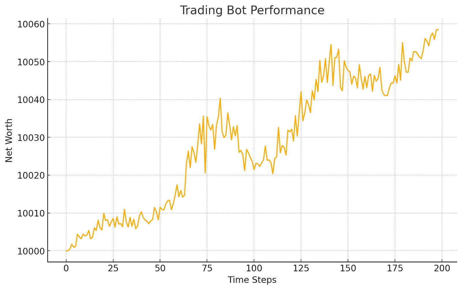
Final Net Worth: $10,058.49The output reflects how the model interacts with the environment, capturing net worth at each step. An upward trend in net worth would indicate successful actions by the model, while a decline suggests suboptimal decisions. If the loop terminated early, it indicates the environment reached a "done" state, concluding the simulation.
Next Steps
Congratulations again, coders! You have created an Reinforcement Learning trading strategy that codes a trading bot to invest in a realistic coding environment.
We encourage you to extend this code with a more complex reward system or more intricately trained DNQ! Go on to experiment with more advanced reinforcement learning models such as PPO (Proximal Policy Optimization) or A2C (Advantage Actor-Critic) to improve trading decision-making. You can also explore neural network architectures like LSTMs or transformers to better capture temporal patterns in stock price data and enhance predictive capabilities.
Thank you so much for tuning in today! Read below to read about using K-Means Clustering to identify similar stocks.
As always, trade smart and stay sharp! Bye!